Micromechanics Plugin for Abaqus/CAE

Overview

Building an accurate material model takes time, and the microstructure is where most of that time goes. Representing it properly means defining a Representative Volume Element, an RVE, that captures the features of the microstructure at the scale you care about. Analysts use it to define the constituents of a system or a microstructure, most often for composites and for the unit cell of the lattice structures common in additive manufacturing.

What is an FE-RVE?

• A finite element (FE) model of a representative volume element (RVE)
• An RVE is a volume of a microstructure large enough to yield the aggregate response of that microstructure
• A periodic RVE applies when the microstructure tessellates under uniform far-field loading, and one tessellating cell (a unit cell) with periodic boundary conditions then gives the aggregate behavior

A plug-in for Abaqus/CAE automates this work, the Micromechanics plug-in. It defines the material properties of the RVE and generates the mesh, which saves a great deal of time against building an RVE by hand for every simulation. We supply it and support its use.

The plug-in also handles far-field loading, which is applied at the boundaries of the simulation domain to model the effect of external forces on the system. You define that loading through periodic or non-periodic boundary conditions, then set up the loads and analysis steps for homogenization of properties or for a far-field load history.

The plug-in takes the repetitive part out of building an accurate simulation and removes a common source of error along the way. Below is what it does.

Download the Micromechanics plug-in and its manual

Extract the plug-in into an abaqus_plugins directory, for instance $HOME/abaqus_plugins, in the Abaqus installation directory. It then appears in the Plug-ins main menu in Abaqus/CAE. The plug-in works with Abaqus/CAE 2016 and later.
> - Extract the plug-in into an abaqus_plugins directory (for instance, $HOME/abaqus_plugins) in the Abaqus installation directory. It then appears in the Plug-ins main menu in Abaqus/CAE.
> - The plug-in works with Abaqus/CAE 2016 and later.

What the plug-in does

The plug-in covers five areas.

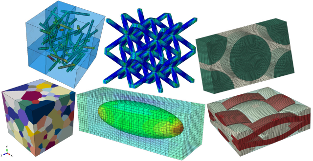
1. Generation of Finite Element Representative Volume Elements (FE-RVE) with specific geometries in a parameterized manner. This includes unidirectional continuous fiber reinforced composites with hexagonal fiber packing, and body-centered or simple-arrayed ellipsoids.

Figure 1: RVE Libraries

2. Automated imposition of boundary conditions on the FE-RVE, including periodic boundary conditions, Taylor boundary conditions where the RVE surface is constrained to the far-field gradient, and Neumann boundary conditions where the far-field flux is applied to the RVE surface. User-defined histories or field histories from a larger-scale analysis can drive these conditions.

Figure 2: RVE Boundary Conditions

3. The study of RVE physics, such as mechanical analysis of both continuum and shell-like microstructures, steady-state heat transfer, and steady-state coupled temperature-displacement.

4. Homogenization of the material properties of the RVE, including elastic stiffness, thermal expansion, shell section stiffness (ABD matrix), thermal conductivity, fully coupled conductivity-stiffness (9x9 constitutive matrix), density, and specific heat.

Figure 3: Homogenization

5. Post-processing tools such as field averaging across the whole RVE and per phase, and histogram generation. These read the simulation results and describe how the system behaves.

Figure 4: Post-Processing

A worked example of the workflow

These capabilities apply across a broad range of workflows. The figure at the end of this section gives one multi-scale example that the plug-in supports.

1. Material calibration step. Characterize the response of a unidirectional composite material at the micro-scale using a fiber-matrix model to predict the transversely isotropic elastic response.
2. Material calibration step. Characterize the response of a textile laminate at the mm-scale using a textile unit cell model with shell-like boundary conditions to obtain the shell section behavior.
3. Study response step. Run an engineering structure simulation at the m-scale to obtain the response of the structure.
4. Study response step. Examine the response of the textile laminate at the mm-scale by analyzing the shell deformation at a point of interest in the engineering structure.
5. Study response step. Examine the response of the fiber-matrix at the micro-scale by analyzing the strain history from a location in the tow, using a fiber-matrix unit cell, all based on the predicted response of the engineering structure.

Figure 5: A typical plug-in workflow

Summary

The FE-RVE plug-in reads the behavior of a composite material from the micro-scale to the macro-scale. It combines material calibration steps with study response steps, so an analyst can examine the stresses and the behavior of the material under a range of conditions. That makes it possible to predict the likely failure modes and to optimize a composite design for the application it has to serve.